The program is designed for the tolerance analysis of two-dimensional (2-D) and three-dimensional (3-D) dimensional chains. The program solves the following problems:
In designing a dimensional chain, the program enables work with standardized tolerance values.
Data, methods, algorithms and information from professional literature and
ANSI, ISO, DIN and other standards are used in calculation.
List of standards: ANSI B4.1, ISO 286, ISO 2768, DIN 7186
![]()
User interface.
![]()
Download.
![]()
Purchase, Price list.
Information on the syntax and control of the calculation can be found in the document "Control, structure and syntax of calculations".
Information on the purpose, use and control of the paragraph "Information on the project" can be found in the document "Information on the project".
A dimensional chain is a set of interdependent dimensions which connect each other to create a geometrically closed circuit. They can be dimensions specifying the mutual position of components on one part or dimensions of several parts in an assembly unit.
A dimensional chain consists of separate partial components
(input dimensions) and ends with a closed component (resulting
dimension). Partial components (A, B, C,…) are dimensions either directly
dimensioned in the drawing or following from previous manufacturing, possibly
assembly operations. The closed component (Z) in the given chain represents the
resulting manufacturing or assembly dimension, which is the result of combining
partial dimensions as a scaled manufacturing dimension, possibly assembly
clearance or interference of a component. The size, tolerance and limit
deviations of the resulting dimension depend directly on the size and tolerance
of partial dimensions. Depending on the mutual position
of the individual components, we differentiate between three types of
dimensional chains:
- Linear chains (1D) – these include only parallel dimensions
- Two-dimensional chains (2D) – the dimensions are distributed in one or
more parallel planes
- Three-dimensional chains (3D) – the dimensions lie in out-of-parallel
planes
This calculation is designed for the tolerance analysis of 2-D and 3-D
dimensional chains.
When solving tolerance relations in dimensional chains, two types of problems occur:
To solve the tolerance relations in dimensional chains, this program uses two
calculation methods:
- "Worst Case" method
- "Monte Carlo" method
The choice of method of calculation of tolerances and limit deviations of
dimensional chain components affects manufacturing accuracy and assembly
interchangeability of components. Therefore, economy of production and operation
depends on it.
The most often used method, sometimes called the maximum - minimum calculation method. It works on the condition of keeping the required limit deviation of a closed component for any combination of real dimensions of partial components, i.e. also upper and lower limit sizes. This method guarantees full assembly and working interchangeability of components. However, due to the demand of higher accuracy of the closed component, it results in too limited tolerances of partial components and therefore high manufacturing costs. The "Worst Case" method is therefore suitable for calculating dimensional circuits with a small number of components or in case that broader tolerance of the resulting dimension is acceptable. It is most often used in piece or small-lot production.
The purpose of the "Worst Case" method is to find the minimum and maximum values that can be achieved by the resulting dimension for a random combination of real input dimensions. The calculation algorithm is based on a gradual testing of all the existing combinations of different (pre-selected) values of input dimensions. In the case of common dimensional chains, the resulting dimension usually reaches its limit sizes only within a certain combination of limit sizes of input dimensions. In tolerance analysis, for the most often solved tasks we can therefore limit ourselves only to testing the combinations of the minimum and maximum dimensions of partial chain components.
In a small percentage of cases, however, the above-mentioned assumption will not hold true and to find the limit sizes of the resulting dimension, it will also be necessary to perform the calculation for the values of the input dimensions lying inside the tolerance interval. In the program, this fact is handled by the optional choice of number of tested values of input dimensions (division of tolerance interval).
Although the selected calculation algorithm guarantees high success in searching for the limit sizes of the resulting dimension for the "Worst Case" method, it may simultaneously lead to disproportionate demands on the duration of the calculation. The speed of the calculation will depend on the total number of calculation cycles performed which are needed to test all the combinations of input dimensions. The number of these cycles depends on the selected division of tolerance interval and grows in a geometric series with an increasing number of partial components of the dimensional chain. It is mathematically described by this relation:
![]()
with:
c ... total of calculation cycles
n ... number of partial components of the dimensional chain
k ... number of tested values of each partial component
From the facts mentioned above, it follows that the "Worst Case" method is designed for solving tolerance relations especially in less complicated dimensional chains with a smaller number of partial components. The practical utilization of the method is limited by the performance of the computer, the number of partial components of the dimensional chain and the selected "precision" of the tolerance interval division.
This method belongs to the statistic methods of dimensional chain calculation. Statistic methods are based on the calculus of probability and assume that in a random selection of components during assembly, the limit values of deviations occur only rarely with more partial components simultaneously, as this is the case of combined probability. The probability of the occurrence of limit value of deviations in manufacturing individual dimensions on one component will be similarly small. With a certain, pre-selected risk of rejection of some components, the tolerances of partial components in the dimensional chain can be increased.
The "Monte Carlo" method guarantees only partial assembly interchangeability, with a low percentage of unfavourable cases (spoilage). With respect to larger tolerances of partial dimensions, however, it results in a decrease in manufacturing costs. It is mainly used in mass and large-lot production, where savings in manufacturing costs outbalance increased assembly and operating costs resulting from incomplete assembly interchangeability of components.
The dimensions of closed component show a certain variance from the mean of the tolerance field. The frequency of occurrence of individual dimensions observes the rules of mathematic statistics. The "Monte Carlo" method is meant to analyse this frequency and determine the expected yield of the manufacturing process.
The "Monte Carlo" method is a simulation method. The algorithm is based on the random generation of input dimensions within selected tolerances according to the rated distribution functions. For this generated set of input dimensions, the calculation of the resulting dimensions is subsequently performed. The process is repeated periodically for the pre-defined number of simulations. The simulation will result in a statistic set of data (resulting dimensions) commonly described by the mean size:
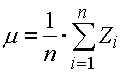
and the standard deviation:
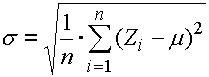
with:
Zi ... value of resulting dimension in the ith cycle of
simulation
n ... total number of simulation cycles
For the evaluation purposes of the frequency of the resulting dimension occurrence, this statistic set is further processed into the form of a histogram.
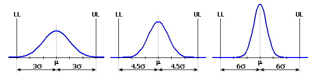
In the case of the "Monte Carlo" method, the expected production yield will be the decisive index for the evaluation of the quality of the dimensional chain design. The production yield gives the expected rate of products meeting the specification requirements, i.e. products with the resulting closed component dimension within the interval set by the required limit sizes. In common engineering, the manufacturing process is usually considered satisfactorily efficient on the level of 3s, i.e. the process with a minimum yield of 99.73%.
The accuracy (informational value) of the ascertained statistic results will depend on the number of simulations performed. It is evident that the quality of the results increases with an increasing number of performed simulations. An optimum number of simulations will depend on the number of input dimensions, their tolerance value and the total complexity of the dimensional chain. In common practice, a value of approximately 30 to 50,000 performed simulations may be considered a reasonable lower limit in the case of final calculations.
This line is used to switch over the system of units for calculation and to select standardized tolerances.
In the list box, select the required system of units for calculation. After switching the units, all values will be automatically recalculated.
When defining the dimensional chain in paragraph [1.1], the tolerance is also set for each dimension. To simplify work, the program is provided with a tool for automatic selection of standardized tolerances.
The program includes a set of basic dimensional tolerances according to ISO, or ANSI. With respect to the type of deviation and applied standard, the tolerances are divided into 5 subsets:
Each subset contains a set of list boxes and buttons in the heading of the workbook. Set the required parameters of tolerance, possibly fits (accuracy level, tolerance field, ..) in the list boxes. Using the buttons, insert the dimensions of the required deviation into the appropriate place in the input table - the line with the active cell.
Tolerances according to ISO are defined by the standard in [mm] and are intended for calculation in SI units. Tolerances according to ANSI are defined in [in] and are intended for calculation in Imperial units. In case of use of standardized tolerances defined in units other than those set in the calculation, the deviations of the dimension will be automatically recalculated and rounded. The ISO 2768 standard is meant for the tolerance of angular dimensions.
The task of the tolerance analysis of the dimensional chain includes the following steps:
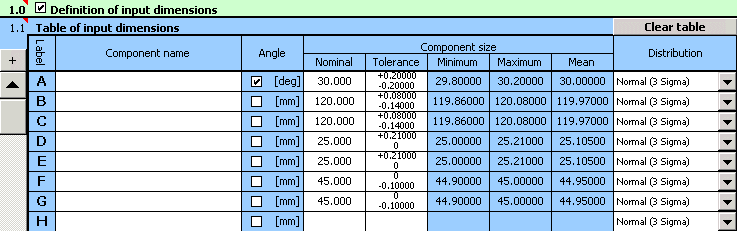
In this paragraph, define the parameters of all partial components of the dimensional chain.
This table is used to define the parameters of the individual input dimensions (partial components) of the dimensional chain. Each line of the table belongs to one partial component. The meaning of the table is obvious from the following description:
Column 1 - Name of component is an optional parameter.
Column 2 – Set the switches to select the type of dimension. Implicitly, a
longitudinal dimension is expected for all components of a dimensional chain;
check the checkbox to set an angular dimension for the selected partial
component. The type of dimension set herein affects the function of the
automatic selection of standardized tolerances.
Column 3 - Set the nominal dimension of partial
component.
Column 4 - Set upper and lower deviation of the
dimension. Press the selected button in the heading of the workbook to insert
the deviations appropriate to the selected tolerance into the table. For the tolerancing of longitudinal dimensions, all the standards
specified herein can be used; tolerances of angular dimensions are standardized
in ISO 2768.
Columns 5..7 – In these columns, the minimum, maximum and mean dimension
of all partial components is calculated.
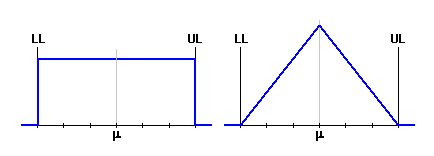
Column 8 - In the list box choose the type of
theoretical frequency distribution. As a standard, normal distribution,
which best matches the real distribution of random process quantities in the
outright majority of cases, is used to describe the manufacturing processes.
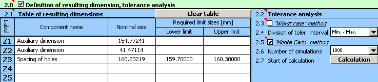
In this paragraph, define the parameters of all closed components of the dimensional chain in Table [2.1]. In Paragraph [2.2], select the required calculation method and set its parameters. Run the calculation using the button on Line [2.7].
This table is used to define the parameters of the individual resulting dimensions (closed components) of the dimensional chain. One line of the table belongs to each dimension. The meaning of the table is obvious from the following description:
Column 1 - Name of component is an optional parameter.
Column 2 – Set the calculation relation used to define the resulting dimension. The formulae used (algorithms) have to observe Microsoft Excel syntax and can contain all mathematic formulae and functions defined by Excel (see Excel help). To mark the input dimensions (partial components) of the dimensional chain, use the symbols consisting of the underscore character and a name of a dimension ("_A", "_B", "_C", ...) in the formulae. Similarly, use the symbols "_Z1", "_Z2", ... for the names of the resulting dimensions. If the calculation relation is defined correctly, the nominal value of the resulting dimension will be calculated in this place in real time. Otherwise, Excel gives the appropriate error value.
Column 3, 4 – Define the required limit sizes of the closed component set by the functional demands of the product. The resulting dimension limits specified herein are optional and are only used for the comparison of the achieved results. In the case of "Monte Carlo" calculation method, the permissible limit values are used to set the expected production yield and reject.
In this paragraph, select the required calculation method and set its parameters. Run the calculation using the button on Line [2.7]. You can find the complete results of the performed tolerance analysis in Paragraph [3].
The purpose of the "Worst Case" method is to find the minimum and maximum values that can be achieved by the resulting dimension for a random combination of real input dimensions. The calculation algorithm is based on a gradual testing of all the existing combinations of different (pre-selected) values of input dimensions. In the case of common dimensional chains, the resulting dimension usually reaches its limit sizes only within a certain combination of limit sizes of input dimensions. In tolerance analysis, for the most often solved tasks we can therefore limit ourselves only to testing the combinations of the minimum and maximum dimensions of partial chain components.
In a small percentage of cases, however, the above-mentioned assumption will not hold true and to find the limit sizes of the resulting dimension, it will also be necessary to perform the calculation for the values of the input dimensions lying inside the tolerance interval. In the program, this fact is handled by the optional choice of number of tested values of input dimensions (division of tolerance interval). Set the required "accuracy" of the division of the tolerance interval in List Box [2.4].
Although the selected calculation algorithm guarantees high success in searching for the limit sizes of the resulting dimension for the "Worst Case" method, it may simultaneously lead to disproportionate demands on the duration of the calculation. The speed of the calculation will depend on the total number of calculation cycles performed which are needed to test all the combinations of input dimensions. The number of these cycles depends on the selected division of tolerance interval and grows in a geometric series with an increasing number of partial components of the dimensional chain.
From the facts mentioned above, it follows that the "Worst Case" method is designed for solving tolerance relations especially in less complicated dimensional chains with a smaller number of partial components. The practical utilization of the method is limited by the performance of the computer, the number of partial components of the dimensional chain and the selected "precision" of the tolerance interval division.
The dimensions of closed component show a certain variance from the mean of the tolerance field. The frequency of occurrence of individual dimensions observes the rules of mathematic statistics. The "Monte Carlo" method is meant to analyse this frequency and determine the expected yield of the manufacturing process.
The "Monte Carlo" Method is a simulation method and belongs to statistic methods. The algorithm is based on the random generation of input dimensions within selected tolerances according to the rated distribution functions. For this generated set of input dimensions, the calculation of the resulting dimensions is subsequently performed. The process is repeated periodically for the pre-defined number of simulations. The simulation will result in a statistic set of data (resulting dimensions) commonly described by the mean size m and the standard deviation s. In the case of the "Monte Carlo" method, the expected production yield will be the decisive index for the evaluation of the quality of the dimensional chain design.
The accuracy (informational value) of the ascertained statistic results will depend on the number of simulations performed. It is evident that the quality of the results increases with an increasing number of performed simulations. An optimum number of simulations will depend on the number of input dimensions, their tolerance value and the total complexity of the dimensional chain. In common practice, a value of approximately 30 to 50,000 performed simulations may be considered a reasonable lower limit in the case of final calculations. Set the required number of simulations in List Box [2.6].
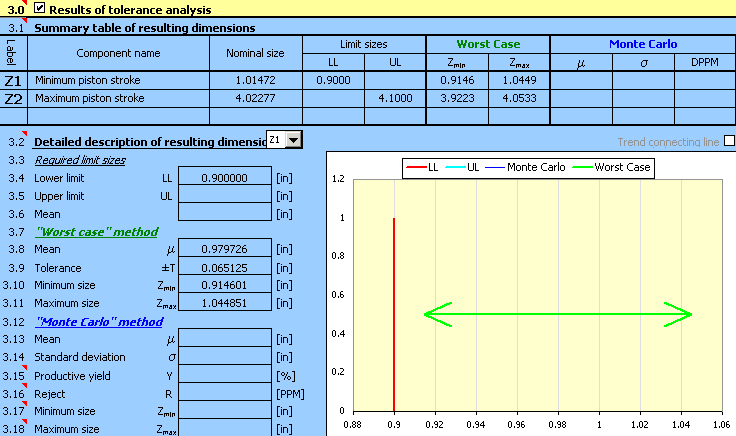
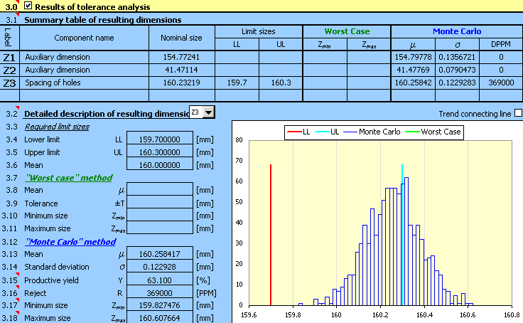
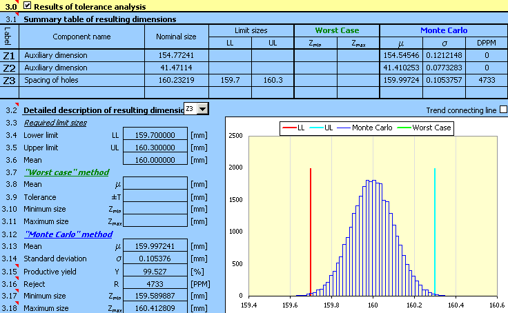
After the end of Calculation [2.7], this paragraph shows the results of the tolerance analysis of the above-defined chain. The paragraph is divided into two parts. In Table [3.1], the basic information regarding all the dimensions defined in Table [2.1] is given in the form of a summary. Paragraph [3.2] presents detailed parameters of the selected resulting dimension in numerical and graphical form.
This table gives a summary of the basic information of all closed components of the dimensional chain defined in Table [2.1]. In the case of a calculation using the "Worst Case" method, the resulting dimension is described using the minimum and maximum value found. In the case of the "Monte Carlo" method, the statistic set specifying the frequency of occurrence of the resulting dimensions is described in the table by mean value, standard deviation and number of rejects per million components produced.
This paragraph presents the detailed parameters of the selected resulting dimension (closed component) of the dimensional chain using the numerical and graphic forms. In the list box, select the required resulting dimension of which you want to show the parameters.
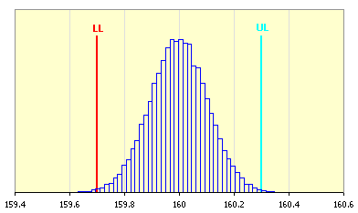
With respect to the calculation method used, the results of the tolerance analysis are divided into two parts. To assess the quality of the dimensional chain design, the limit sizes that can be achieved by the resulting dimension [3.10, 3.11] are decisive for the "Worst Case" method. In the case of the "Monte Carlo" method the decisive index is given by the expected production yield [3.15] or the number of rejects per million pieces produced [3.16]. The enclosed histogram shows the frequency of occurrence of the individual dimensions.
The productive yield specifies the expected rate of products meeting the requirements of the specification, i.e. products with a resulting dimension of closed component within the interval given by the required limit sizes. In common engineering, the manufacturing process is usually considered satisfactorily efficient at the level of 3s, i.e. the process with a minimum yield of 99.73%.
Rejection of the manufacturing process gives the expected number of unsuitable products, i.e. products with the resulting dimension of closed component outside the interval given by the required limit sizes. In common engineering, the manufacturing process is usually considered satisfactorily efficient at the level of 3s, i.e. the process with maximum number of 2,700 rejected pieces per million produced.
The limit sizes specified herein have only an informative character. These limits do not determine the real limit values which can be achieved by the resulting dimension. They only specify the minimum and maximum value of the dimension found during simulation calculation within the selected number of simulations. To find the real limit sizes, it is necessary to use the "Worst Case" calculation method.
To illustrate the problems of the tolerance analysis of dimensional chains, help is completed with practical examples of the use of this calculation:
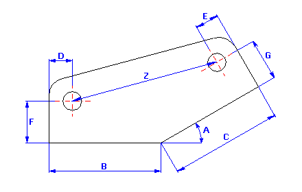
For the eccentric crank gear of a piston compressor (see the picture), ascertain the:
If we start from the graphic illustration of the dimensional chain
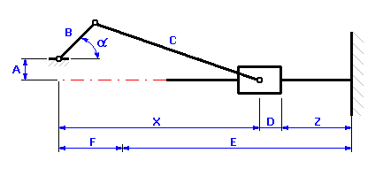
we can describe the rate of the piston stroke in the case of the given kinematical mechanism by the relation of:
![]()
where the position of the piston against crankshaft axis X is a kinematical quantity dependent on the angle of orientation of the crankshaft, a. For the eccentric crank gear illustrated in the previous picture, the following relation can be used to set the position of the piston:
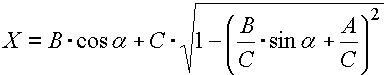
The limit positions of the piston against the crankshaft axis are obvious from the following diagram
and can be described by these relations:
![]()
The solution of the task of the tolerance analysis of the kinematical mechanism can be divided into the following steps:
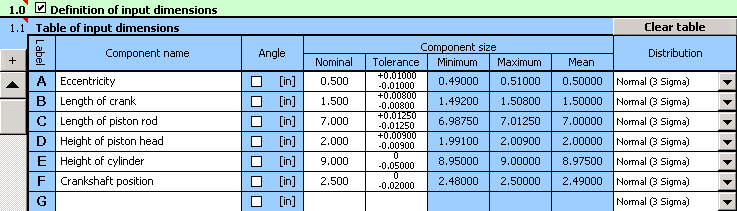
1) In Table [1.1] we will define all the input dimensions (partial components) of the dimensional chain.
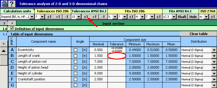
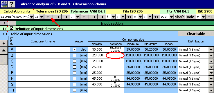
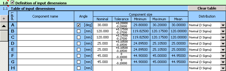
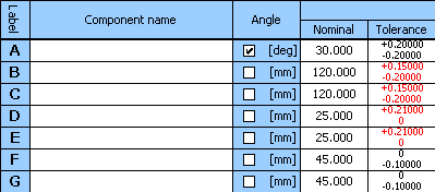
2) For the individual dimensions we will further set the rated production tolerances. For dimensions B, C and D, the standardized symmetrical tolerances according to ANSI B4.1 in accuracy level 13 are rated. To set them in the table, we can use the function of automatic tolerance selection.
3) In Table [2.1] we will define the parameters of the resulting dimensions (closed components) of the dimensional chain. The calculation relations for the minimum and maximum piston stroke defined in the previous paragraph have to be modified into the form (syntax) required by Excel. Therefore, in the second column of the table, we will set the relation "=_E+_F-_D-((_C+_B)^2-_A^2)^0.5" for the minimum piston stroke and the relation "=_E+_F-_D-((_C-_B)^2-_A^2)^0.5" for the maximum piston stroke.
4) In Line [2.3], check the switch next to the "Worst Case" calculation method. In List Box [2.4], further select the "roughest" division of tolerance interval ("Min. - Max." item) which is sufficient for the given task.
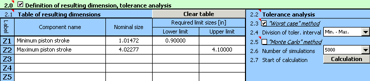
5) Press the button on Line [2.7] to run the calculation (tolerance analysis) of the dimensional chain. The limit values of the stroke can be found in Paragraph [3].
The procedure of solving this task will be similar to the previous one and can be divided into the following steps:
1) The input dimension will be defined in Table [1.1] similarly to example A in steps 1) and 2).
2) The angle of crankshaft orientation for which we intend to set the piston stroke will be defined as a constant "Z1" in the first line of Table [2.1]. In the second line of Table "Z2", set the relation for the calculation of the stroke. The above-mentioned calculation relation has to be modified into the form (syntax) required by Excel:
"=_E+_F-_D-(_B*COS(RADIANS(_Z1))+_C*(1-(_B/_C*SIN(RADIANS(_Z1))+_A/_C)^2)^0.5)"
3) In Line [2.3], check the switch next to the "Worst Case" calculation method. In List Box [2.4], further select the "roughest" division of the tolerance interval ("Min. - Max." item).
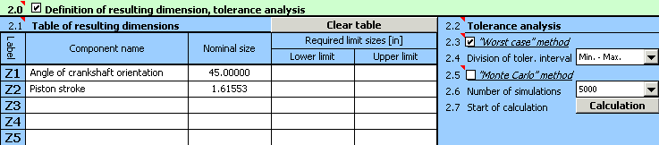
4) Press the button on Line [2.7] to run the calculation. The parameters of the stroke for the given angle can be found in Paragraph [3].
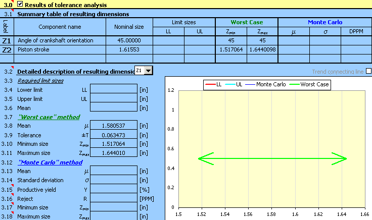
5) To set the stroke for a different value of orientation angle, it will be enough to change the angle size in Table [2.1] and recalculate the task using Button [2.7].
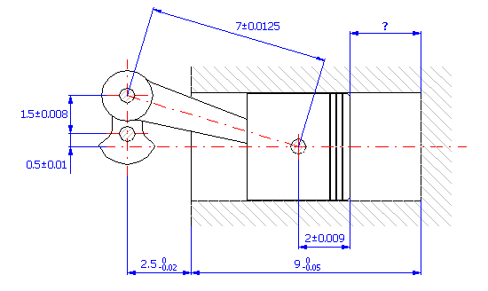
For the component (see the picture) design, the production tolerances of the dimensions are such that the required distance 160±0.3 mm between the centres of orifices is maintained for at least 99.5% of the manufactured components.
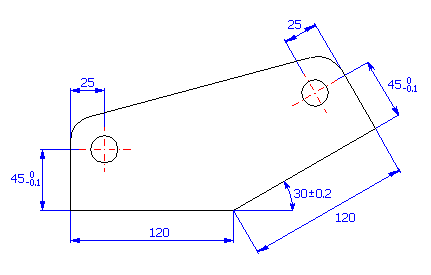
If we start from the graphical illustration of the dimensional chain
we can describe the resulting dimension for the given component using this relation:
![]()
where the following relations will hold for the auxiliary variables X, Y:
![]()
![]()
If the task was solved using the traditional "Worst Case" method, it would be necessary to use tolerances at approximately accuracy level 4 for dimensions B, C, D and E so that the required tolerance of the resulting dimension was kept. It is obvious that production with this accuracy would be disproportionately expensive. Therefore, it will be more convenient to use the statistic method of calculation in this case. These methods enable the manufacture of the component with significantly higher tolerances upon the occurrence of a small (pre-determined) percentage of rejects.
The solution of the task of the dimensional chain design can be divided into the following steps:
1) In Table [1.1], define all input dimensions (partial components) of the dimensional chain.
2) Further set the production tolerances for all dimensions. For dimensions with strictly set tolerances, set the rated dimensional deviations in the input table.
For the remaining dimensions, select a tentatively symmetrical tolerance at accuracy level 12.
3) In the list boxes, in the last column of the table, select a normal division with a production process capability level of 3s for all dimensions.
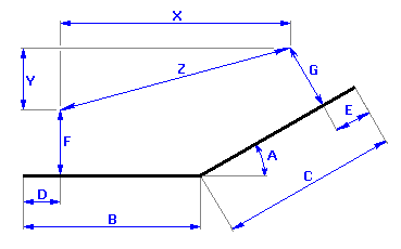
4) In Table [2.1], define the parameters of the resulting dimension (closed component) of the dimensional chain. To facilitate work and increase clear arrangement, we will divide the calculation relation into three parts (see above). We will use the first two lines of the table to define the auxiliary dimensions; the parameters of the searched resulting dimensions will be placed on Line "Z3". The above-mentioned calculation relations have to be modified in the form (syntax) required by Excel. Therefore, set the following text into the appropriate lines of the second column of the table:
Line 1 "Z1" ..... "=_B-_D+(_C-_E)*COS(RADIANS(_A))-_G*SIN(RADIANS(_A))"
Line 2 "Z2" ..... "=(_C-_E)*SIN(RADIANS(_A))+_G*COS(RADIANS(_A))-_F"
Line 3 "Z3" ..... "=(_Z1^2+_Z2^2)^0.5"
5) On line [2.5] check the switch next to the "Monte Carlo" calculation method. In List Box [2.6] further set the required number of simulations. To speed up the designing process, set smaller numbers of simulations in the initial steps of designing.
6) Press the button on Line [2.7] to run the calculation (tolerance analysis) of the dimensional chain. The parameters of the resulting dimension can be found in Paragraph [3].
7) Expected production yield [3.15], better stated number of rejects [3.16] will be the decisive factor for the assessment of the design quality. The task assignment prescribes the maximum permissible number of 5,000 rejects per million pieces produced. The achieved results are higher by order of magnitude; therefore the designed tolerances are not suitable.
For an unsuitable design, the next logical step could be decreasing the sizes of the manufacturing tolerances used. On a closer view of the design, however, we discover that the main problem is not the selected size of tolerances, but rather the improper centring of the design. In the case of an optimally designed dimensional chain the mean dimension [3.13] should be close to the required dimension [3.6].
8) Therefore, in the next step we will adjust the position of the tolerance fields of dimensions B, C, D and E, while maintaining the originally designed values of the tolerances. By repeated adjustments of the deviations of the individual dimensions with a subsequent recalculation of the results, we will gradually achieve the solution
for which the design will be centred
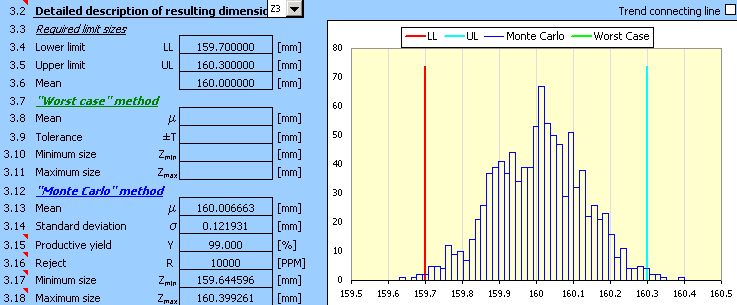
9) Although the design is already well centred, the required production yield has not yet been achieved. In the next step it will be necessary to decrease the tolerances designed tentatively in Step 2). After selecting the tolerances of dimensions B and C in accuracy level 11 and the centring of design, we will achieve the suitable solution
which meets the functional requirements set by the task assignment.
Information on setting of calculation parameters and setting of the language can be found in the document "Setting calculations, change the language".
General information on how to modify and extend calculation workbooks is mentioned in the document "Workbook (calculation) modifications".
^