Design and optimization of linear dimensional chain using statistical "RSS" method.

For the component (see picture), design the manufacturing tolerances of dimensions so that the permissible deviation ±0.0013 in for the technologically resulting dimension is not exceeded.

Solution of problem.

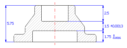
If we start from the diagram of the dimensional chain

we can describe the resulting dimension for the given component using the relation Z = C - A - B.

If the problem were solved using the common "Worst Case" method, it would be necessary to use tolerance at approx. accuracy level 4 for dimensions B and C to keep the required tolerance of the resulting dimension. It is obvious that production with such accuracy level would be unreasonably expensive. In this case it will therefore be much more advantageous to use the statistical method of calculation. This method enables manufacturing of a component with significantly greater tolerances, at the cost of a low (pre-selected) percentage of spoilage.

Design of dimensional chain.

The solution to the task of dimensional chain design and optimization can be divided into the following steps:

1) Using the above-mentioned relation, we will define the dimensional chain in table [1.1]. 

2) We will further set the required manufacturing tolerances for individual dimensions. We will set the appropriate deviations for dimension A required by the task.

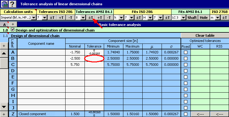
For the remaining dimensions we will tentatively select symmetrical tolerance at accuracy level 8.

Note: Although this step is not absolutely essential, it will ensure that the optimized tolerances are designed to the proper ratio. During the design of individual tolerances, the mutual ratio of their dimensions given by values set in the input part of the table will be kept.

3) In column 8 of the table, check the switch with dimension A, the tolerance of which is strictly given.

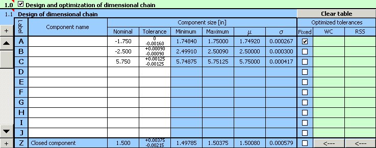
4) In paragraph [1.3] set the required limit values of the resulting dimension.

5) In list box [1.7] choose the "Centring and optimization" method, in list [1.8] set the required accuracy (number of decimal places) designed by the tolerance.

6) With respect to the various methods of machining applicable during production of the component, set the minimum allowed tolerance to accuracy level 6 in the list box [1.9]. 

Hint: You will find a table of achieved manufacturing accuracies for different methods of machining in the workbook "Tolerances and fits".

7) In list box [1.10] choose the required production yield 99.9%, i.e. manufacturing process with maximum number of 1000 rejects per million manufactured components.

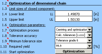
8) Start optimization of the dimensional chain using the button in line [1.11].

9) The resulting design parameters are shown in paragraph [2.10],

optimized deviations of manufacturing processes are shown in column 10 of table [1.1].

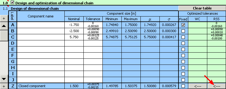
10) The designed tolerances can of course be further adjusted. Using the button on the bottom line of the table, transfer the optimized values of tolerances into the input part of the table. There, while keeping the tolerance sizes, we can e.g. finely tune the designed deviations to a more suitable shape.

Calculation results for this adjustment will be the same as the result achieved for the optimized tolerances.

Final note.

The solution designed here will not of course be the only suitable solution to the problem and need not therefore be the ideal solution. When choosing a suitable solution, it is necessary to assess the relationship between the chosen sizes of manufacturing tolerances and expected manufacturing process yield. By increasing the applied tolerances we will achieve a decrease in direct costs connected with machining of the components, but it will result in an increase in losses due to the increased occurrence of faulty products. It is necessary to choose the resulting solution so that the total manufacturing costs are as low as possible.

For comparison, the following table shows the values of expected production yield for normalized tolerances of dimensions B and C.