The program is designed to solve the most common problems in fluid mechanics.
The program solves problems in the area of:
1. Hydrostatics
2. Stationary fluid discharge through hole
3. Stationary discharge - overflows (ISO 1438, Swiss Engineers, Hansen, Bazin, Frese)
4. Stationary flow of viscous fluid - constant pipe cross section with output nozzle / diffuser
5. Stationary flow of fluid - various pipe cross sections
6. Water hammer
Calculations include determination of Reynolds number, viscosity, laminar and turbulent flow losses for various materials, and dozens of types of loss coefficients.
The calculations use data, procedures, algorithms and information from literature, standards, and company catalogues.
[1] Mechanika tekutin - ČVUT (Prof. Ing. Jan Ježek, DrSc, Ing. Blanka Váradiová,
CSc., Ing Josef Adamec, CSc)
[2] Mechanika tekutin, Sbírka příkladů - ČVUT (Ing. Milan Peťa)
[3] Strojně technická příručka (Svatopluk Černoch)
[4] Mechanika tekutin, VŠB-TU Ostrava (Janalík J., Šťáva P.)
[5] Textbook of Machine Design (R.S. KHURMI, J.K. GUPTA)
[6] A TEXTBOOK OF FLUID MECHANICS AND HYDRAULIC MACHINES (Dr. R.K. Bansal)
[7] Roloff / Matek - Maschinenelemente, Normung, Berechnung, Gestaltung
[8] Fluid mechanics, seventh edition (Frank M. White)
[9] 2500 Solved problems in fluid mechanics and hydraulics
(Jack Evett, Cheng Liu)
[10] Handbook of hydraulics (Brater, King, Lindell, Wei)
ISO 1438:2017
Hydrometrie — Měření průtoku vody v otevřených korytech pomocí tenkostěných
přelivů
Hydrometry — Open channel flow measurement using thin-plate weirs
Hydrometrie — Mesure de debit dans les canaux découverts au moyen de déversoirs
a paroi mince
![]() User interface.
User interface.
![]()
Download.
![]()
Purchase, Price list.
Information on the syntax and control of the calculation can be found in the document "Control, structure and syntax of calculations".
Information on the purpose, use and control of the paragraph "Information on the project" can be found in the document "Information on the project".
Fluid mechanics is an extensive field of study of fluid motion and action. The Fluid Mechanics calculations include many frequently solved problems.
Dynamic Viscosity
The dynamic viscosity µ (µ = "mi") is a measure of the viscosity of a fluid
(fluid: liquid, flowing substance).
The higher the viscosity, the thicker (less liquid) the fluid; the lower the
viscosity, the thinner (more liquid) the fluid is.
SI unit of dynamic viscosity: [µ] = Pascal-second (Pa*s) = N*s/m² = kg/m*s
The kinematic viscosity ν (ν = "nu") is the dynamic viscosity of
the medium µ divided by its density ρ (ρ = "Ro").
Equation: ν = µ / ρ
SI unit of kinematic viscosity: [ν] = m²/s
Frequently used units are Stokes (St) and Centistokes (cSt).
Conversion:
1 Stoke (St) = e-4 * m²/s = 1 cm²/s
1 cSt = e-6 m²/s = 1 mm²/s
An approximate formula is used to calculate the viscosity as a
function of temperature:
µ ~ µ20 * exp(C * (293 / TK - 1))
µ20 ... Dynamic viscosity at 20°C
C ... Coefficient for a given fluid
TK ... Temperature in Kelvin
The dimensionless Reynolds number is the basic parameter that
determines the viscous behavior of all Newtonian fluids.
It depends not only on the mean velocity but also on the characteristic
dimension of the fluid flow (diameter d or dh), dynamic viscosity, and density.
Re = v * d *
r /
µ, respectively Re = v * dh *
r /
µ
for non-circular cross-sections
v ..... Velocity
d ..... Diameter
r ... Density
µ ..... Dynamic viscosity
dh ... Hydraulic diameter
dh = 4 * S/O
S ... Cross-sectional area
O ... Wetted circumference
For a circular cross section d = dh.
Empirical expression:
µ /
µ20 = exp(C * (293 / T°K
- 1))
µ ... Dynamic viscosity
µ20 ... Dynamic viscosity for 20°C
C ... Coeficient
T ... Temperature
Differences from ideal fluid flow:
1) Losses occur when some of the mechanical energy is converted to
heat.
2) The velocity is not uniformly distributed in the cross section.
3) Fluid motion can be laminar (Re=Re,cr<2300) or in most cases turbulent
(Re>3000).
Q = v1 * S1 = v2 * S2
Q ... Flow rate
v1, v2 ... Velocity in cross sections 1 and 2
S1, S2 ... Area in cross sections 1 and 2
g*h1 + p1/Ro + k1*(v1^2)/2 = g*h2 + p2/Ro + k2*(v2^2)/2 + ez(1-2)
g ... Acceleration of gravity
Ro ... Density
h1, h2 ... Height
p1, p2 ... Pressure
v1, v2 ... Velocity
ez(1-2) ... Energy of loss
ez(1-2) = (Zeta + Lambda * (L/dh)) * (v^2/2)
Zeta ........ Local loss coefficient (input, cross section change, valve....)
Lambda ... Friction loss coefficient
L ............. Length
dh ........... Diameter
v ............. Velocity
Lambda ... Friction loss coefficient
Laminar flow (Re<2300):
Lambda = 64 / Re
Turbulent flow (Re>=2300):
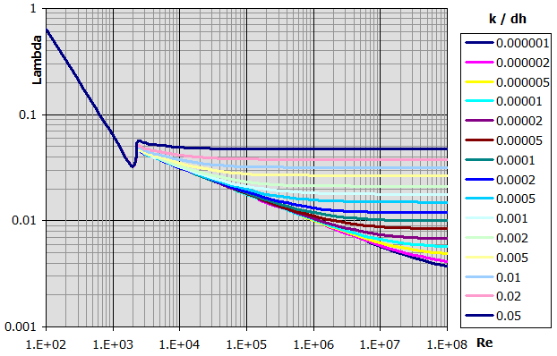
Methods of Lambda calculation:
Smooth Pipe:
Lambda = 0.3164 / (Re^0.25) ....... Blasius
Lambda = 1 / (2 * Log10(Re * Lambda^0.5) - 0.8)^2 ......... Nikurdas
Lambda = (1.8 * Log10(Re) - 1.5)^-2 .......... P.K.Konakov
Rough Pipe:
Lambda = 0.1 * (100 / Re + kr)^0.25 ....... Altus
Lambda = 1 / (-2 * Log10(2.51 / (Re * Lambda^0.5) + 0.27 * kr))^2 ........
Colebrook - White
Lambda = 8 * ((8 / Re)^12 + 1 / (a + b)^1.5)^(1/12) ....... Churchill
a = (2.457 * Log(1 / ((7 / Re)^0.9 + 0.27 * kr)))^16
b = (37530 / Re)^16
Lambda = 1 / (2 * Log10(1 / kr + 1.138))^2 ....... Gottingen formula
Lambda = 1 / (2 * (Log10((dh/2) / k) + 1.74)^2) ........ Karman formula
kr = k / dh
k ..... Roughness (Height of Roughness)
dh ... Diameter (Hydraulic diameter)
Lambda = 4 * f
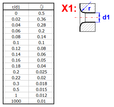
zetaI ... Input loss coefficient (Roundness)
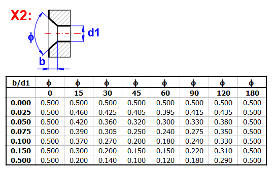
zetaI ... Input loss coefficient (Chamfer)
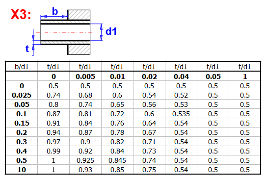
zetaI ... Input loss coefficient (Extrusion)
zetaB ... Loss coefficient (Bending)
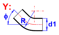
zetaB =(0.131 + 0.16 * (d1 / R)^3.5) * (Fi / 90)
zetaI ... Loss coefficient (Transition)
Nozle, delta<10: ZetaI = (Lambda / (8 * SIN(delta/2))) *
(1 - (S2/S1)^2)
Nozle, delta>=10: ZetaI = Table aproximation
Diffuser: ZetaI = (S2/S1 - 1)^2 * SIN(MIN(delta;90))
zetaV ... Valve loss coefficient
The table below can be used for an approximate orientation:
ZetaS ... Loss coefficient for pipeline splitting
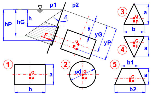
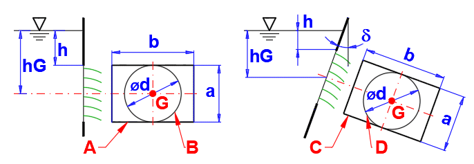
Hydrostatic Force:
F = ((p1 - p2) + Ro * g * hG) * S
p1, p2 ... Pressure
g ... Acceleration of gravity
Ro ... Density
hG ... Depth of the centre of gravity of the surface
S ... Surface
1. yP = y+(2*a + 3*y)/(a + 2*y) * (a/3)
2. yP = y+(8*y + 5*a) / (2*y + a) * (a/8)
3. yP = y+(4*y + 3*a) / (3*y + 2*a) * (a/2)
4. yP = y+(2*y + a) / (3*y + a) * (a/2)
5. yP = y+(2*y*(b1 + 2*b2) + a*(b1 + 3*b2)) / (3*y*(b1 + b2) + a*(b1 + 2*b2)) * (a/2)
a ...
Acceleration
g ... Acceleration of gravity
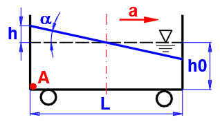
h = L / 2 * tan(a)
L ... Wessel length
Pressure on A:
pA = Ro
* (g^2 + a^2)^0.5 * (h0 + dh) * COS (a)
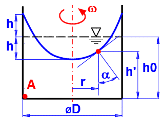
w = 2 * p * n / 60
n ... Revolution
h = (w^2 * (D / 2)^2) / (4 * g)
w ... Angular speed
D ... Diameter
g ... Acceleration of gravity
Pressure on A:
pA = 0 -
r * g * (-h0 +
h) + 0.5 * r
* h^2 *
w^2
h' = h0 - h + r^2 *
w^2 / (2 * g)S
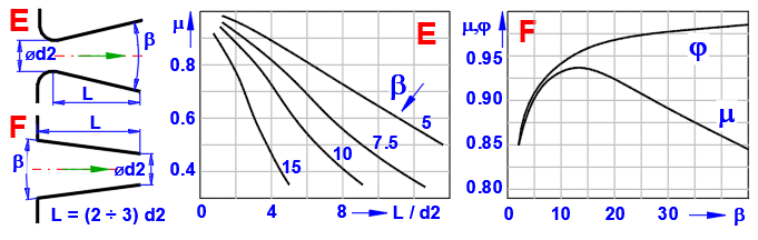
The actual flow rate of a real fluid differs from the theoretical values for the ideal fluid. When the fluid flows out through an opening (or a short nozzle), the contact with the wall is small; thus, the energy dissipation will be small as well. Therefore, it is possible to consider the fluid as inviscid and correct the theoretical results with the following correction factors.
j = v / vt
v .... Actual discharge velocity
vt ... Theoretical discharge velocity
a = S2' /
S2
S' ... Actual fluid flow cross section
S .... Cross-section of the orifice
m = a * j
= Q / Qt
Q .... Actual volumetric flow
Qt ... Theoretical volumetric flow
v2t = ((2 * g * (h1 + (p1 - p2) / Ro)
/ (1 - (S2 / S1)^2))^0.5
g ... Acceleration of gravity
Ro ... Density
p1, p2 ... Pressure
S1, S2 ... Area
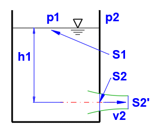
v2 = j * v2t
Qt = S2 * v2t
Q = a * S2 * j * v2t = m * Qt
Coefficient m in relation to Re for type A outlet without nozzle
Re = v2t * d / n
n ... Kinematic viscosity
For large openings (top edge close to the surface and the ratio of opening height to centre of gravity depth close to one) a non-linear distribution of the discharge velocity must be considered.
Rectangular Opening
Q = m * b * (2 * g)^0.5 * ((h + a)^(3/2) - h^(3/2))
Circular Opening
Q = m * p * r^2 * (2
* g * hG)^0.5 * (1 - 1/32 * (r / hG)^2 - 5/1024 * (r / hG)^4)
r = d / 2
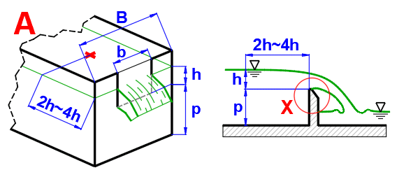
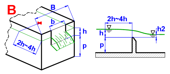
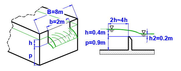
From the perspective of hydraulics, the spillway is a large discharge opening, with no top wall above the beam (Figure A). The spillway may be ideal if the level behind the spillway is lower than the spillway edge, or imperfect (flooded) if the level behind the spillway is higher (Figure B). Ideal spillways are used to determine the amount of fluid flowing. Depending on their shape, spillway edges may be rectangular, triangular, trapezoidal, or circular.
The level h must be measured at a sufficient distance before the spillway (usually 2h - 4h). Above the spillway, the level is lower because part of the positional energy has already been converted into kinetic energy.
Volumetric Flow Rate (ISO 1438)
Q = Cd * (2/3) * (2 * g)^0.5 * be * he^(3/2)
Cd ... Discharge coefficient
g ... Acceleration of gravity
be ... Effective width
he ... Effective overflow height
he = h + 0.001
be = b + kb
Q = 2/3 * Cd * b * h * (2 * g *
h)^0.5
b ... Width
h ... Overflow height
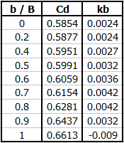
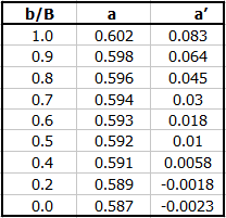
Cd = a + a' * (h / p)
in dependence on b/B
Flow Coefficient (Society of
Swiss Engineers)
Cd = 0.615 * (1 + (1 / (1000 * h + 1.6))) * (1 + 0.5 * (h / p)^2)
Flow Coefficient (Hansen)
Cd = 0.61706 / (1 - 0.35815 * (h^3)^0.5)
Flow Coefficient (Bazin)
Cd = (0.6075 + 0.045 / h) * (1 + 0.55 * (h / (h + p))^2)
Flow Coefficient (Frese)
Cd =
(0.5755+0.017/(h+0.18)-0.075/(b+1.2))*(1+(0.25*(b/B)^2+0.025+0.0375/((h/(h+p))^2+0.02))*(h/(h+p))^2)
Volumetric Flow Rate (ISO 1438)
Q = f * Cd * (2/3) * (2 * g)^0.5 * be * he^(3/2)
f ... Flooded coefficient
for h/p=0.5, f =1.007 * ((0.975 - h2/h)^1.45)^0.265
for h/p=1.0, f =1.026 * ((0.960 - h2/h)^1.55)^0.242
for h/p=1.5, f =1.098 * ((0.952 - h2/h)^1.75)^0.22
for h/p=2.0, f =1.155 * ((0.950 - h2/h)^1.85)^0.219
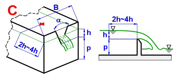
Spillway with Triangular Cross-Section
Volumetric Flow Rate (ISO 1438)
Q = Cd * (8/15) * TAN(alfa/2) * (2 * g)^0.5 * he^(5/2)
he ... Effective spillway height
A frequent task to solve for constant cross section piping, bends, valves, etc. The universal Bernoulli's equation with the use of loss factors is used for the solution.
Calculation of flow rate, velocities, losses, and power in pipes of constant cross section.
Calculation of Discharge Velocity:
v2 = ((2 * g * (H +((p1 - p2) / (Ro * g))))/((ZetaI + Lambda * ((L1-L2) / dh1) +
ZetaBV) * (dh2 / dh1)^4 + (1 + ZetaO)))^0.5
g ..... Acceleration of gravity
H ..... Surface height
p1, p2 ... Pressure
dh1, dh2 ... Hydraulic diameter
L1,L2 ... Length
Ro ... Density
Lambda ... Friction loss coefficient
ZetaI ... Input loss coefficient
ZetaBV ... Loss coefficient of bends+valves
ZetaO ... Nozzle / Diffuser loss coefficient
ZetaO ... Nozzle/Diffuser Loss Coefficient
Numerical integration (100 steps), sequential calculation of Sx, vx, Rex, Lambdax, hzx and from the total loss height hz the zetaO coefficient related to the discharge velocity v2.
For diffuser and delta angle > 10°
ZetaO = ((S2 / S1) - 1)^2 * SIN(delta)
The Bernoulli equation is used for the calculation, using the loss coefficients to calculate the output velocity vo in the form:
Calculation of flow rates, velocities, losses, power in pipelines of various cross sections and number of branches.
A = 2 * g * (v0^2 / (2 * g) + (p1 - p2) / (Ro * g) + H)
B(i) = (Zeta(i) + Lambda(i) * L(i) / dh(i)) * n(i) * (So / S(i))^2
vo = (A / (1 + SB(i)))^0.5
[i = 1 .... 15]
g ..... Acceleration of gravity
H ..... Aurface height
p1, p2 ... Pressure
v0 ... Surface velocity
dh(i) ... Hydraulic diameter
L(i) ... Length
n(i) ... Number of parallel pipes
So ... Otput cross section
S(i) ... Pipe cross section i
Ro ... Density
Lambda ... Friction loss coefficient
Zeta ... Sum of loss coefficients zetaI, zetaB, zetaV
The calculation of the loss coefficients is described above.
Chart example
When regulating the flow of fluid through a pipeline, a non-stationary flow is created. As the flow rate decreases, more pressure is created in front of the valve than behind it. In the case of long pipelines transporting fluid, a rapid (emergency) closure of the pipeline can lead to an increase in the pressure, which can damage the pipeline.
When the pipeline is closed, the kinetic energy of the fluid is gradually used to compress the fluid or deform the pipeline. The shock wave travels through the pipeline at the speed of sound in the given fluid in the direction B->A and back to A->B.
t = 2 * L / a
L ... Length of the pipe
a ... Speed of sound
at = (K / Ro)^0.5
K ..... Bulk modulus of fluid
Ro ... Density
a = (K / Ro)^0.5 / (1 + (K*d) / (E*th))^0.5
E ... Modulus of elasticity of the pipe material
d ... Diameter of the pipe
th ... Pipe wall thickness
a = (K/Ro)^0.5 / (1 + 2 * (K/E) * ((D^2 + d^2) / (D^2 - d^2)))^0.5
E ... Modulus of elasticity of the pipe material
d ... Inner diameter of the pipe
D ... Pipe outer diameter
A. Perfectly rigid pipe
p = Ro * (v1 - v2) * at
B. Thin-walled pipe
p = Ro * (v1 - v2) * a
v1, v2 ... Fluid velocity
p = Ro * L * (v1 - v2) / t
The calculations cover some frequently solved problems in fluid mechanics. If your task falls within the range of problems addressed by this calculation, proceed as following:
1. In paragraph [1], select the fluid, set its parameters (if required), and
define environmental parameters.
2. Select the appropriate task and fill in the known input values.
3. The calculations are in the form of a mathematical model of the given
problem. Therefore, if the result of the calculation is to be one of the input
parameters, it is necessary to iterate over this parameter.
In this paragraph, you set the calculation units, select and set the fluid and the environment properties.
In the dropdown list, select the required system of calculation units. Upon switching the units, all calculation values will be updated to reflect your selection.
Select the required fluid. The values in the list are for barometric pressure. To enter your own fluid parameters, uncheck the check box on the right.
By unchecking the check box on the right, you can enter either the speed of sound or the bulk modulus of elasticity.
By unchecking the check box on the right, you can enter either kinematic or dynamic viscosity.
For most calculations, a zero altitude setting is sufficient. However, there may be problems where different barometric pressures or different accelerations of gravity must be taken into account.
The standard acceleration of gravity is considered at sea level for 45° latitude.
The Reynolds number Re is a dimensionless parameter that defines the transition from laminar to turbulent flow. For Re < 2300 the flow is laminar, for Re > 3000 the flow is almost always turbulent.
The critical Re therefore determines the method of calculation and thus the values of the loss coefficients.
Some frequently solved problems in hydrostatics.
Enter the required values as shown in the figure.
Marking points:
G ... Centre of gravity of the area
P ... Point of action of the force
By unchecking the check box on the right, you can enter your own value for the pressure above the surface and the pressure outside the vessel.
Area perpendicular to the surface: delta=0
Area parallel to the surface: delta=90
The total force on the surface S. It has a point of action at P.
The distance of the centre of gravity of the surface from the free surface of the fluid.
The distance of the centre of pressure from the free surface of the fluid.
The calculation does not solve the situation when the level hits the bottom of the vessel.
The calculation does not solve the situation when the level hits the bottom of the vessel.
Calculation of the steady flow of fluid through an opening.
The actual flow rate of the real fluid differs from the theoretical values for the ideal fluid. When the fluid flows out through an opening or short nozzle, the contact with the wall is small; thus, the energy dissipation will be small as well. Therefore, it is possible to consider the fluid as inviscid and correct the theoretical results with the following correction factors.
By unchecking the check box on the right, you can enter your own value for the pressure above the surface and the pressure outside the vessel.
If the tank is not cylindrical, it is possible to enter the transverse surface directly by unchecking the check box on the right.
If the opeing is not circular, it is possible to enter the area of the hole manually by unchecking the check box on the right.
For comparison purposes only. It does not include any losses.
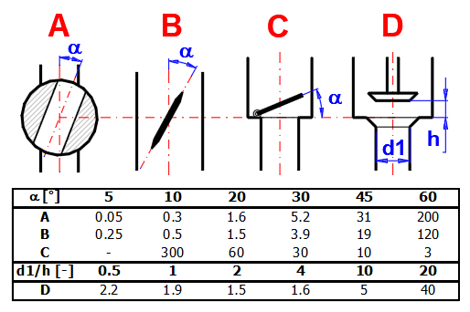
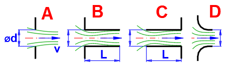
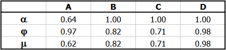
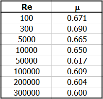
For the discharge through a hole without a nozzle (figure A), the discharge coefficient can be determined as a function of the Reynolds number Re. The first value on the left is the calculated Re. On the right you can see the discharge coefficient, which can be used instead of the standard value of 0.62.
Select the appropriate coefficients according to the type of the outlet (A-F) according to the given table and graphs.
To enter the discharge coefficient manually (product of [3.11] and [3.12]), uncheck the check box on the right.
For large openings (the upper edge near the surface and the ratio of the hole height to the depth of the center of gravity is close to one), a nonlinear distribution of the discharge velocity must be considered.
Use the same discharge coefficient as for a small opening [3.13].
From the perspective of hydraulics, the spillway is a large discharge opening with no top wall above the beam (Figure A). The spillway may be ideal if the level behind the spillway is lower than the spillway edge, or imperfect (flooded) if the level behind the spillway is higher (Figure B). Ideal spillways are used to determine the amount of fluid flowing. Depending on their shape, spillway edges may be rectangular, triangular, trapezoidal, or circular.
The level h must be measured at a sufficient distance before the spillway (usually 2h - 4h). Above the spillway, the level is lower because part of the positional energy has already been converted into kinetic energy.
In the calculation, the boundary conditions for which the calculations are defined are then listed to the right of the input cells.
There are a number of formulas and procedures for the calculation of rectangular spillways (Fig. A), or for the calculation of the flow coefficient Cd, which are reported in the literature. Therefore, we present them as well for comparison.
The height above the spillway h is usually measured at a distance of 2h ~ 4h from the spillway (eliminating the drop in level above the spillway).
If the level at the outlet affects the water flow (Figure B), it is possible to use this calculation with that the overflow parameters are defined in Section A.
The value of the coefficient as a function of p and the ratio h2/h is given in the green cell.
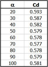
If the area of the cut-out is relatively small compared to the cross-sectional area of the inflow, it is possible to use experimentally determined Cd dependent only on the angle of the cut-out.
A frequent task to solve for constant cross section piping, bends, valves, etc. The universal Bernoulli equation with the use of loss coefficients is used for the solution. Calculation of flow rate, velocities, losses, and power in constant cross section pipe.
Fill in all dimensional and pressure parameters. You can use the calculations on the right to estimate the loss coefficients. It is possible to choose a negative pressure (p2>p1) and it is possible to choose a negative height (H<0), but in any case it is necessary to keep the sense of fluid flow from the inlet to the outlet.
The pressure p1=p2 from paragraph [1.0] is used as the default value. Enter the pressure inside the vessel p1 and the ambient pressure p2 by unchecking the check box on the right.
The level height must be greater than the value on the right.
If the outlet is higher than the level, enter the height H as a negative value (must be compensated by overpressure p1>p2).
In case p1<p2, the external overpressure must be compensated by the level height H.
If the pipe is not circular, you can enter the value of the pipe area and wetted perimeter after unchecking the check box on the right. The hydrodynamic diameter dh is then determined from these values using the formula dh = 4 * S / C, which is then used in the calculations.
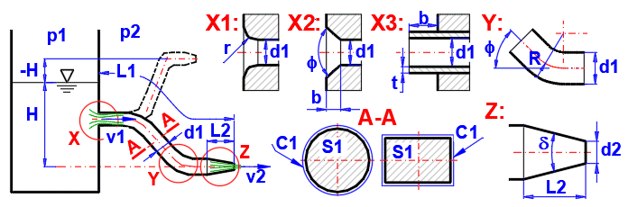
Indicated in the figure as cross section A-A.
Select the appropriate pipe material from the list. The default roughness value in [mm/in] on the next line is the average of the range indicated in brackets. After unchecking the chec box on the right, you can enter your own value.
Based on the pipe roughness "k" and the coefficient "Re", a number of formulas for calculating the friction loss coefficient for turbulent flow are given in the technical literature. Select the appropriate calculation from the list.
The most commonly used calculation is "C. Colebrook - White", which also covers hydraulically smooth pipes (k=0). Details in the help.
The design of the Lambda friction loss coefficient depends on Re and at the same time the calculation of Re depends on the Lambda friction loss coefficient (calculation of the flow velocity).
The design value is automatically transferred to the input cell.
After unchecking the check box on the right, you can enter your own value.
Select the input coefficients according to the calculations/recommendation on the right.
Marked as X1, X2, X3 in the picture.
It is the sum of all coefficients for all possible losses in the pipe (bends, valves...).
The loss coefficient of the pipe bend can be found by the calculation on the right. The loss coefficients of the valves can be roughly estimated from the figure.
Select if the pipe has a nozzle / diffuser at the end.
If d1>d2 (dh1>dh2), the loss proposal is used for the nozzle. If d1<d2, the loss proposal is used for the diffuser.
If the pipe is not circular, you can enter the value of the pipe area and wetted perimeter after unchecking the check box on the right. The hydrodynamic diameter dh is then determined from these values using the formula dh = 4 * S / C, which is then used in the calculations.
Indicated in the figure as cross section A-A.
Enter the length of the nozzle / diffuser. It must be less than the length of the pipe L1.
It is calculated from the values of dh1, dh2 and L2.
Estimation based on loss integration is used for nozzle (d1> d2) and diffuser (delta <10). For difuser and delta>10, when the fluid flow is separated from the pipe wall, the relation zetaO = ((S2 / S1) - 1)^2 * SIN(delta) is used.
It gives the ratio between the altitude and pressure energy at the intlet and the kinetic energy of the output fluid flow.
These power parameters allow the evaluation of the pipeline.
It is applicable:
Pp + Ph = Pz + Po
or
Pp + Ph + Pv = Pz + Po for paragraph [6.0]
Flow rates are often given in different units, independent of the calculation units. Therefore, the conversion of the most commonly used units is provided below.
The Bernoulli equation is used for the calculation using loss coefficients to
calculate the output velocity vo.
Calculation of flow rates, velocities, losses, power in pipes of various cross
sections and number of branches.
Fill in the conditions at the input to the pipeline.
It is possible to choose a negative overpressure (p2>p1) ant it is possible to choose a negative height (H<0), but in any case, it is necessary to keep the sense of fluid flow from the inlet to the outlet.
The pressure p1=p2 from paragraph [1.0] is used as the preset value. Uncheck the check box on the right to enter the pressure inside the vessel p1 and the outside pressure p2.
The velocity of the fluid (kinetic energy) before entering the pipe. In most solved problems (large vessel relative to the volume of the pipeline), it is possible to ignore the velocity and use a zero value. For example, it will be non-zero in the case of a piston that pushes fluid through a pipe.
The level height must be greater than the value on the right.
If the output hole is higher than the level, enter the height H as a negative value (must be compensated by overpressure p1>p2).
In case p1<p2, the external overpressure must be compensated by the level height H.
Based on the pipe roughness "k" and the coefficient "Re", a number of formulas for calculating the friction loss coefficient for turbulent flow are given in the technical literature. Select the appropriate calculation from the list.
The most commonly used calculation is "C. Colebrook - White", which also covers hydraulically smooth pipes (k=0). More details cain be found in the help.
The sum of the pressure energy potential (p2-p1), the fluid pressure
potential (H), and the kinetic energy of the fluid (v0) at the entrance to the
pipe.
Usually, the energy level is expressed in meters of fluid column. Select the
units in which the energy level is to be expressed on the right.
In the graph below, it is indicated by the blue horizontal line (Fig2 - A).
For comparison purposes only. Does not include any losses.
It gives the ratio between the altitude and pressure energy at the intlet and the kinetic energy of the output fluid flow.
These power parameters allow the evaluation of the pipeline.
It is applicable:
Pp + Ph = Pz + Po
or
Pp + Ph + Pv = Pz + Po for paragraph [6.0]
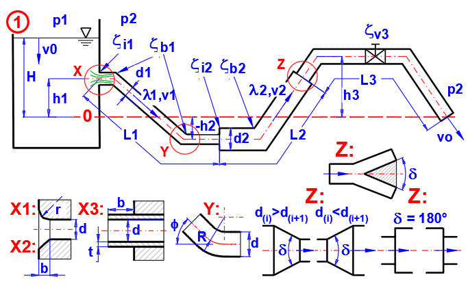
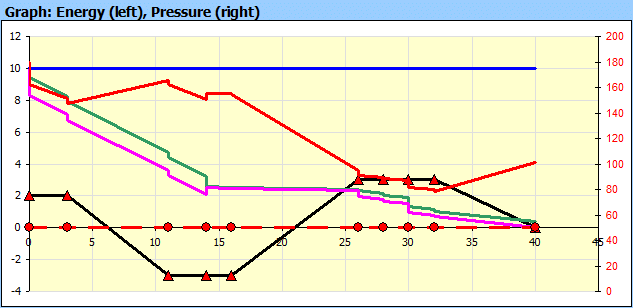
Graph description (Fig.2):
Line A: Total Energy Line. It gives the sum of the energies (height-Eh,
pressure-Ep and kinematic-Ev) of the fluid at the inlet to the pipe..
Line B: Sum of the height (Eh) and pressure (Ep) energies
Line C: Energy Height (Eh)
Line 0: Zero line relative to the end of the pipe
Curve 1: Loss height hz (losses in the different parts of the pipeline)
Curve 2: Pressure in the pipe (scale on the right in kPa or psi)
Curve 3: Kinematic height
Curve 4: Height points of the beginning of each section relative to the zero
line
Fill in the values for each pipe section in the table one by one (one row for each section).
It is possible to choose a simplified or detailed approach, or a combination of both.
Simplified (Fig2. Ver1):
The individual sections are divided according to the pipe diameter and all loss
coefficients (inlet, bend, valve ...) in one section are summarized into one
coefficient (column H), which is applied at the beginning of the relevant
section.
Detailed (Fig2. Ver2):
The pipeline is divided into sections so that the relevant loss coefficient
(column H) is always at the beginning of the section. This will give you a more
detailed graph [6.19]. The overall results (Q, vo ...) are identical..
Select the number of consecutive sections to be solved (1-15).
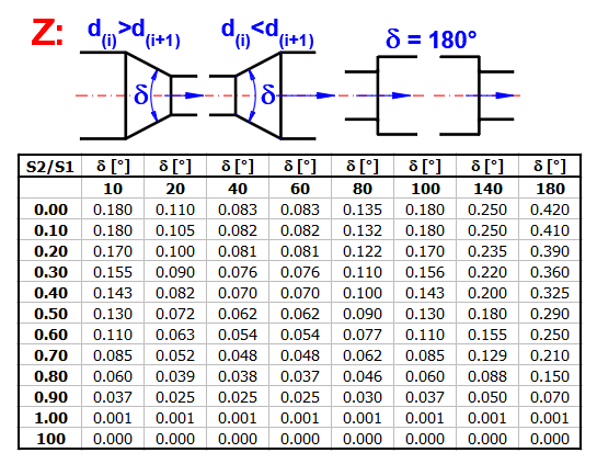
It is possible to split one pipe into two or more pipes. Alternatively, merge several pipes into one. (Fig. Detail Z)
Height of the beginning (start) of the pipe section above (or below) outlet (end) point of the last section (zero line).
The length of the particular section.
Enter the diameter. If the pipe is not circular, enter the hydraulic diameter
dh (see the description of Surfaces in paragraph E).
Pressing the "V" key copies the value from the first line to the others.
If the check box on the right is checked, the area is calculated from the circular cross section of diameter d from the column on the left (D).
For non-circular cross-section pipe, uncheck the check box on the right and
enter the cross-sectional area (E) and the hydraulic diameter dh in the diameter
cell (D).
dh = 4 * S / C
where:
S ... Cross-sectional area
C ... Wetted circumference
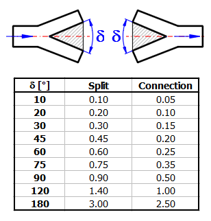
Angle of narrowing / widening of the transition between two sections (Fig1. Det.Z). In case of splitting the pipe into two branches, then it is the angle between the pipes.
The corresponding proposed loss factor ZetaI is on the right (column G).
Based on the area ratio (column E) and the chamfer (column F) between the two sections, a loss coefficient at the beginning of the section is proposed (More details can be found in the theoretical part of the help). The loss coefficient in the case of pipeline branching is proposed in a similar way.
With the "=>" button you can transfer the proposed design to column H, which is used in the calculation.
The sum of all loss factors in the relevant pipe section.
ZetaI .... Input losses, losses by section change ( design column G)
ZetaB ... Bending losses (calculation in previous paragraph [5.0])
ZetaV ... Valve losses (table in previous paragraph [5.0])
To calculate the real pipe, it is necessary to specify the roughness of the pipe. Use the table below for reference. Press the "V" button to copy the value from the first row to the others.
- Hydraulically smooth pipe (0-0) mm / (0-0) in
- Steel - Continuous seamless pipe (0.03-0.1) mm / (0.00118-0.00394) in
- Welded new steel pipe (0.05-0.1) mm / (0.00197-0.00394) in
- Welded steel tubes corroded (0.15-0.5) mm / (0.00591-0.01969) in
- Welded steel sheet - air pipes (0.5-0.8) mm / (0.01969-0.0315) in
- Steel sheet riveted (1-6) mm / (0.03937-0.23622) in
- Brass and aluminium tubes pure drawn (0.0015-0.01) mm / (0.00006-0.00039) in
- Glass, plastic (0.0015-0.01) mm / (0.00006-0.00039) in
- Cast iron new pipe (0.1-0.3) mm / (0.00394-0.01181) in
- Cast iron old pipe (1-4.5) mm / (0.03937-0.17717) in
- Rubber tubing (0.01-0.03) mm / (0.00039-0.00118) in
- Plywood (0.025-0.1) mm / (0.00098-0.00394) in
- Ceramic (0.45-6) mm / (0.01772-0.23622) in
- Bricks with cement smear (0.8-6) mm / (0.0315-0.23622) in
- Concrete (0.8-9) mm / (0.0315-0.35433) in
Reynolds number Re (See help for details - Theory)
Characterizes the flow of a viscous fluid, which depends not only on the mean
velocity but on the characteristic dimension of the fluid flow (diameter d or
dh), dynamic viscosity and density.
It is used to calculate the friction loss coefficient Lambda (column K).
Design of Friction loss coefficient Lambda. Depends on Re (column J). However, the calculation of Re is backwards dependent on the flow velocity (for which knowledge of Lambda is required). Therefore, there is a sequential iteration of values.
The proposed value is automatically transferred to the cell on the right
(column L), which is used for the calculation.
After unchecking the check box on the right, you can enter your own value of the
friction loss coefficient.
Friction loss coefficient Lambda. It is necessary for the calculation of the flow velocity. If the check box on the right is checked, the design value (column K) is used.
Unless you have an important reason for a different value, please use the design value.
Press the "V" button to copy the value from the first row to the others.
The velocity of the fluid in a given section of pipeline.
In the N,O column, select which values you want to display and their units. The selection of units is linked to line [6.8].
hIBV ... Sum of losses ( input, bend, valve) for the given section
hF ...... Frictional losses for a given section
h-A, h-B, h-C ... Losses from the beginning of the pipe sequentially at points
A,B,C (Fig.2)
v(pd) ... Energy of the flowing fluid (dynamic pressure)
p-A, p-B, p-C ... Absolute pressure at points A,B,C
When regulating the flow of fluid through the pipe, a non-stationary flow is created. As the flow rate decreases, more pressure is created in front of the valve than behind it. In the case of long pipelines transporting liquid, a rapid (emergency) closure of the pipeline can lead to an increase in the pressure which can damage the pipeline.
When the pipe is closed, the kinetic energy of the fluid is gradually used to compress the fluid or deform the pipe. The shock wave travels through the pipe at the speed of sound in the fluid in the direction B->A and back to A->B.
Press the button to load the parameters from paragraph [5.0].
Fill in the input parameters as shown on the picture.
Select the pipe material.
After unchecking thecheck box on the right, you can enter a custom value.
When the valve is fully closed v2=0.
Two cases can occur:.
1. Valve closing time t > T-shock wave travel time [7.14,7.21]
As the valve closing time decreases, the pressure increases.
2. Valve closing time t < T-shock wave travel time [7.14,7.21]
The pressure remains constant at its highest intensity.
It is defined in paragraph [1.0]
The theoretical speed of sound [7.20] depends on the density of the material and the bulk elasticity of the liquid. For real pipes, the speed of sound propagation decreases depending on the dimensions and material of the pipe.
Approximate calculation of viscosity and density of a liquid as a function of temperature.
Enter the temperature of the selected liquid.The density and viscosity are suggested based on the temperature. The calculation is approximate with an accuracy of +- 6% in the temperature range 0-100°C (32-212°F).
Press the button to move the density and viscosity values to paragraph [1.0].
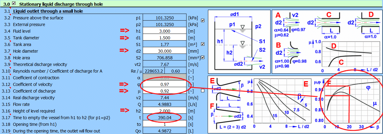
Paragraph [3.0] - Calculation of the level decrease time from h1 to h2.
Vessel defined according to the figure.
Liquid: water, 20°C, p1=p2=atmospheric pressure (Paragraph [1.0]).
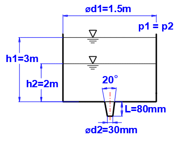
Enter the input values as shown in the figure, and get the coefficients j and m from the graph F. The time for the level decrease is on line [3.17].
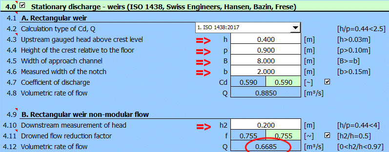
Paragraph [4.0]. Flow calculation using a flooded spillway.
The spillway defined according to the figure.`
Calculation method according to ISO 1438.
Enter the input values as shown in the figure. The resulting flow rate for the flooded spillway is on line [4.12].
Paragraph [5.0]. Pipe diameter calculation for the required fluid flow.
Definition of pipe dimensions and loss coefficients according to the figure.
Required flow rate 100L/s = 0.1 m³/s
Input losses = 0.5, bend+valve losses = 5*0.3 + 2*1.5 = 4.5
Cast iron pipe (new), roughness k=0.2mm
Method of calculation of loss coefficient Lambda: Colebrook - White
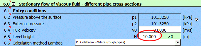
Liquid: water, 20°C, p1=p2=atmospheric pressure (Paragraph [1.0])
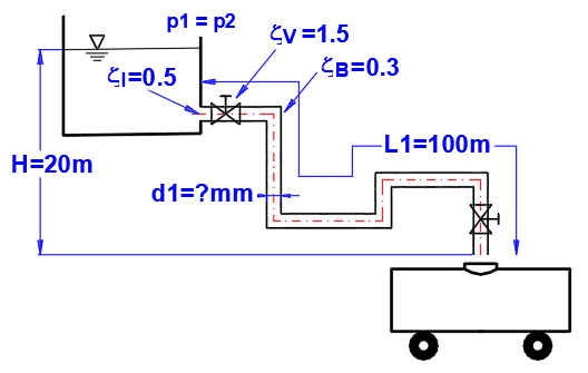
Enter all known parameters and gradually change the value of d1 [5.5] to achieve the desired flow rate Q = 0.1 m³/s
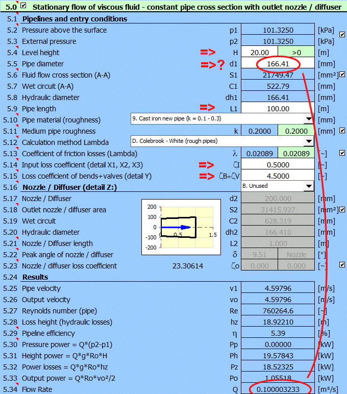
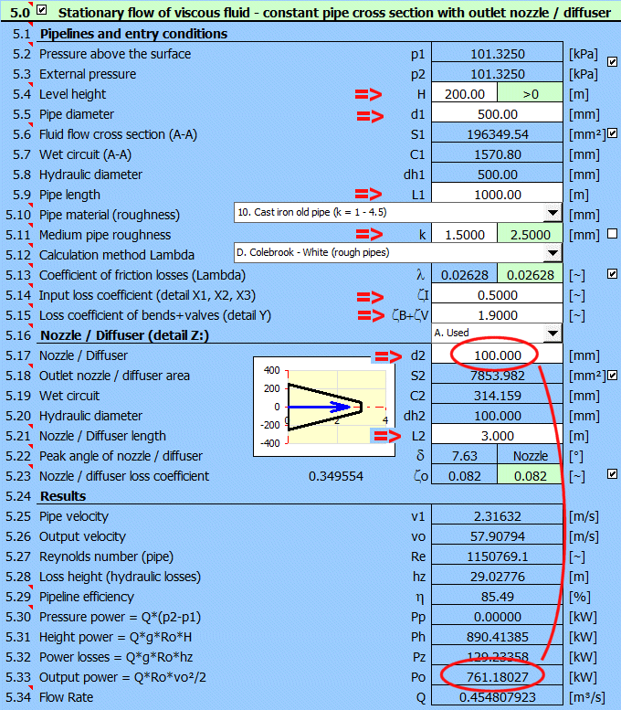
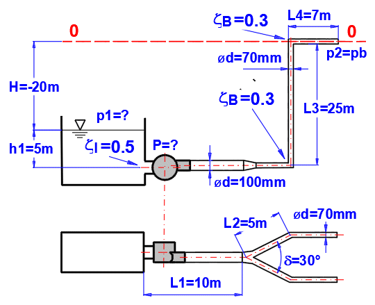
Paragraph [5.0]. Calculation of the current output at the end of the nozzle for the specified diameter. Determining for which nozzle diameter the maximum power is achieved.
Definition of the dimensions and loss coefficients of the pipe as shown in the figure.
Input losses = 0.5, bend+valve losses = 2*0.2 + 1.5 = 1.9
Cast iron pipe, roughness k=1.5 mm
Method of calculating the loss coefficient Lambda: Colebrook - White
Liquid: water, 20°C, p1=p2=atmospheric pressure (Paragraph [1.0])
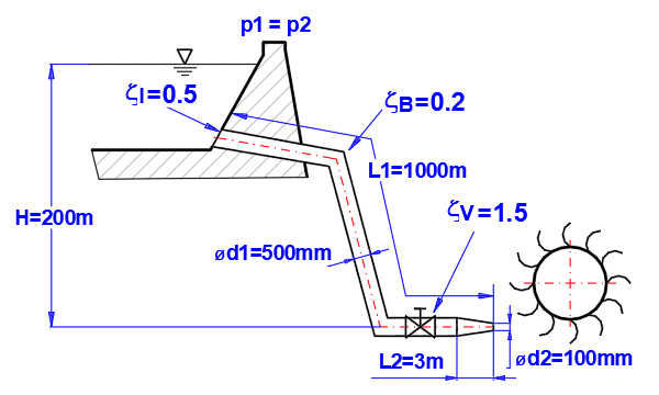
Enter all known parameters. The power of the liquid stream at the end of the nozzle is Po = 761kW [5.33]
To find the maximum power, change the nozzle diameter d2 gradually. Maximum power Po = 1162kW for d2=157.6mm.
At the same time, the efficiency is reduced from 85.5% for d2=100mm to 61.8% for d2=157.6mm.
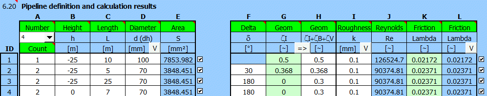
Paragraph [6.0]. Calculation of detailed progression of pressure and losses in the pipeline, calculation of fluid velocities and flow rates.
Pipeline defined according to figure and table, where:
ID ... Section number (1-9)
L ... Lengths of each section
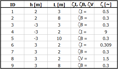
ZetaI, ZetaB, ZetaV ... Losses at the beginning of the section ( input, change of section, bend, valve)
Pipe material: cast iron, roughness k=1.5mm
Method of calculating the loss coefficient Lambda: Colebrook - White
Fluid: water, 20°C, p1=p2=atmospheric pressure (Paragraph [1.0])
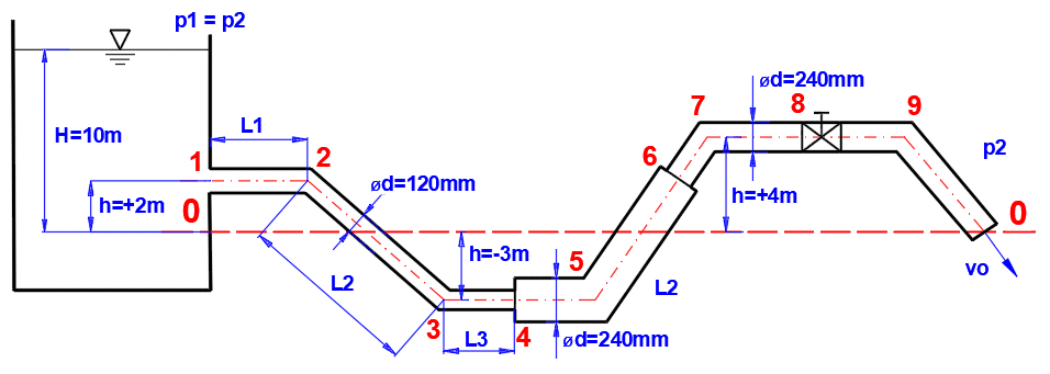
Definition of conditions:
Define the pipe parameters (A-number of pipes, B-height relative to zero line, C-length of sections, D-pipe diameter, F-transition angle between different pipe diameters, H-uniform loss coefficients, I-pipe roughness)
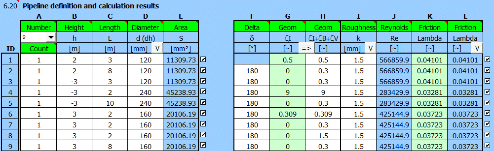
Results:
Detailed course of pressure and losses:
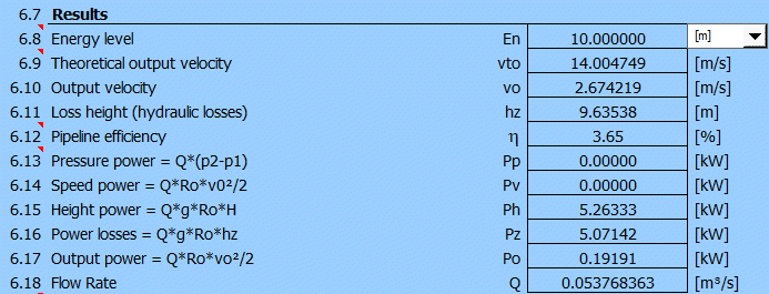
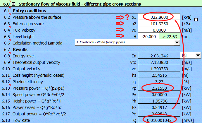
Paragraph [6.0]. Calculation of pump power for pumping water up to 25m. The required flow rate is 10l/s.
Piping defined as shown in the figure.
L ... Lengths of individual sections
ZetaI, ZetaB ... Losses (entry, change of cross-section, pipe splitting, bending)
Pipe material: steel pipe, roughness k=0.1mm
Method of calculating the loss coefficient Lambda: Colebrook - White
Fluid: water, 20°C, p2=atmospheric pressure (Paragraph [1.0])
Define the pipeline parameters (A-number of pipes, B-height relative to zero line, C-length of sections, D-pipe diameter, F-pipe split angle, H-individual loss coefficients, I-pipe roughness)
The loss for pipe splitting is at G2.
Enter all known parameters and gradually change the pressure value p1 [6.2] to reach the desired flow rate Q = 0.01 m³/s [6.18]
The required pump power can then be found on the line [6.13] Pp=2.22kW.
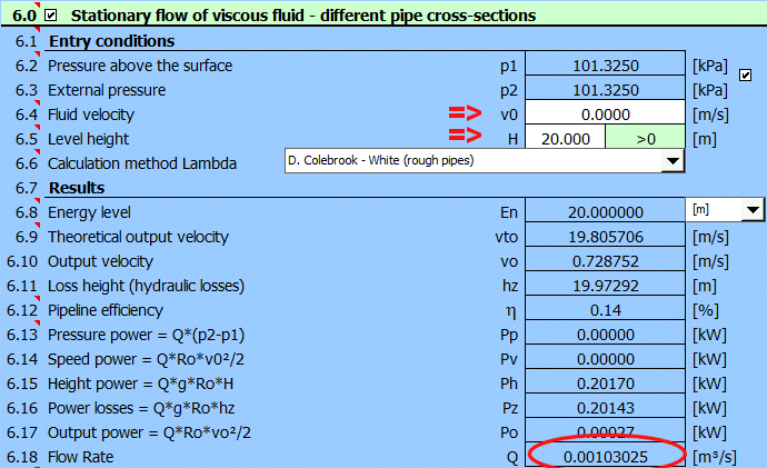
Paragraph [6.0]. Calculation of water flow in the shower.
Pipes and shower defined according to the figure:
L ... Lengths of the individual sections
ZetaI, ZetaV, ZetaB ... Losses ( input, valve, bend)
Pipe material: steel pipe, roughness k=0.1mm
Lambda loss coefficient calculation method: Colebrook - White
Liquid: water, 20°C, p1=p2=atmospheric pressure (Paragraph [1.0])
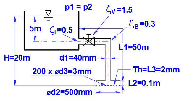
Define the parameters of the pipe and shower with 200 holes.
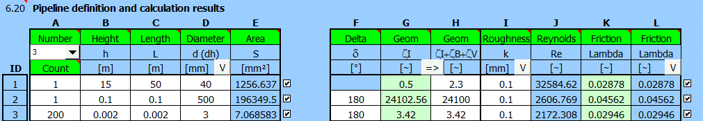
Specify the level height. The water flow through the shower Q=1L/s is on line [6.18].
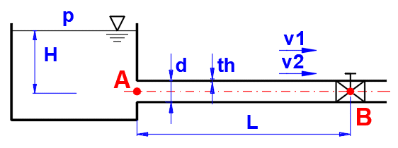
Paragraph [7.0]. Calculation of hydraulic hammer during emergency closure of the pipeline from Example 4. Checking stress in the pipeline.
You can use the "[5.0] >> [7.0]" button to define parameters.It will load the values from paragraph [5.0].
Next, enter the material, set the pipe wall thickness to 20 mm and the valve closing time to 2 seconds.
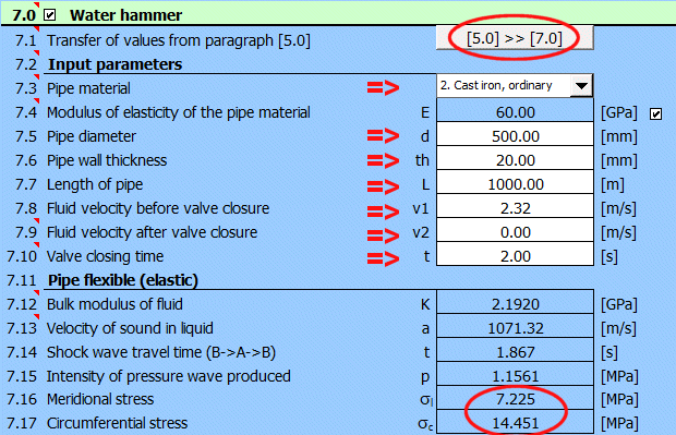
Compare the stress increase [7.16, 7.17] for the valve closing time for t<1.86 s.
Information on setting of calculation parameters and setting of the language can be found in the document "Setting calculations, change the language".
General information on how to modify and extend calculation workbooks is mentioned in the document "Workbook (calculation) modifications".
Literature:
[1] Mechanika tekutin - ČVUT (Prof. Ing. Jan Ježek, DrSc, Ing. Blanka Váradiová, CSc., Ing Josef Adamec, CSc)
[2] Mechanika tekutin, Sbírka příkladů - ČVUT (Ing. Milan Peťa)
[3] Strojně technická příručka (Svatopluk Černoch)
[4] Mechanika tekutin, VŠB-TU Ostrava (Janalík J., Šťáva P.)
[5] Textbook of Machine Design (R.S. KHURMI, J.K. GUPTA)
[6] A TEXTBOOK OF FLUID MECHANICS AND HYDRAULIC MACHINES (Dr. R.K. Bansal)
[7] Roloff / Matek - Maschinenelemente, Normung, Berechnung, Gestaltung
[8] Fluid mechanics, seventh edition (Frank M. White)
[9] 2500 Solved problems in fluid mechanics and hydraulics (Jack Evett, Cheng Liu)
[10] Handbook of hydraulics (Brater, King, Lindell, Wei)
Standards:
ISO 1438:2017
Hydrometrie — Měření průtoku vody v otevřených korytech pomocí tenkostěných přelivů
Hydrometry — Open channel flow measurement using thin-plate weirs
Hydrometrie — Mesure de debit dans les canaux découverts au moyen de déversoirs a paroi mince
^